Fibonacci Heap

Introduction

The Fibonacci heap data structure serves a dual purpose.

1. It supports a set of operations that constitutes what is known as a “mergeable heap”
2. Several Fibonacci-heap operations run in constant amortized time.

Basic Operations

1. $MAKE-HEAP()$: creates and returns a new heap containing no elements
2. $INSERT(H, x)$: inserts element $x$, whose key has already been filled in, into heap $H$.
3. $MINIMUM(H)$: returns a pointer to the element in heap $H$ whose key is minimum
4. $EXTRACT-MIN(H)$: deletes the element from heap $H$ whose key is minimum, returning a pointer to the elements.
5. $UNION(H_1, H_2)$: creates and returns a new heap that contains all the elements of heaps $H_1$ and $H_2$. Heaps $H_1$ and $H_2$ are “destroyed” by this operation.
6. $DECREASE-KEY(H, x, k)$: assigns to element $x$ within heap $H$ the new key value $k$, which we assume to be no greater than its current key value.
7. $DELETE(H, x)$: deletes element $x$ from heap $H$.

Comparison with Binary Heap

Procedure	Binary Heap	Fibonacci Heap
$MAKE-HEAP()$	$\Theta(1)$	$\Theta(1)$
$INSERT(H, x)$	$\Theta(\lg n)$	$\Theta(1)$
$MINIMUM(H)$	$\Theta(1)$	$\Theta(1)$
$EXTRACT-MIN(H)$	$\Theta(\lg n)$	$O(\lg n)$
$UNION(H_1, H_2)$	$\Theta(n)$	$\Theta(i)$
$DECREASE-KEY(H, x, k)$	$\Theta(\lg n)$	$\Theta(1)$
$DELETE(H, x)$	$\Theta(\lg n)$	$O(\lg n)$

From the above table, we can conclude that Binary heap works fairly well if $UNION$ operation is not needed. But in cases $UNION$ operation is necessary, normal binary heap starts to perform poorly.

Fibonacci heaps, on the other hand, have better asymptotic time bounds than binary heaps for the $INSERT$, $UNION$, and $DECREASE-KEY$ operations. Note that all running time in the above table are amortized time bounds instead of worst-case per-operation time bounds.

Fibonacci Heaps in Theory and Practice

Theoretically speaking, Fibonacci heaps are especially desirable when the number of $EXTRACT-MIN$ and $DELETE$ operations is small relative to the number of other operations performed. Such situation arises in many applications. For example, some algorithms for graph problems may call $DECREASE-KEY$ once per edge. For dense graphs, which have many edges, the $\Theta(1)$ amortized time of each call of $DECREASE-KEY$ adds up to a big improvement over the $\Theta(\lg n)$ worst-case time of binary heaps. Fast algorithms for problems such as computing minimum spanning trees and finding single-source shortest paths make essential use of Fibonacci heaps.

From a practical point of view, however, the constant factors and programming complexity of Fibonacci heaps make them less desirable than ordinary binary (or k-ary) heaps for most applications, except for certain applications that manage large amounts of data. Thus, Fibonacci heaps are predominantly of theoretical interest.

Both binary heaps and Fibonacci heaps are inefficient in $SEARCH$ operation; it can take a while to find an element with a given key. For this reason, operations such as $DECREASE-KEY$ and $DELETE$ that refer to a given element require a pointer to that element as part of their input.

Like several other data structures that we have seen, Fibonacci heaps are based on rooted trees. We represent each element by a node within a tree, and each node has a key attribute.

Structure of Fibonacci Heaps

A Fibonacci heap is a collection of rooted trees that are min-heap ordered. That is, each tree obeys the min-heap property: the key of a node is greater than or equal to the key of its parent. The following is the figure from Introduction to Algorithms, Third edition.

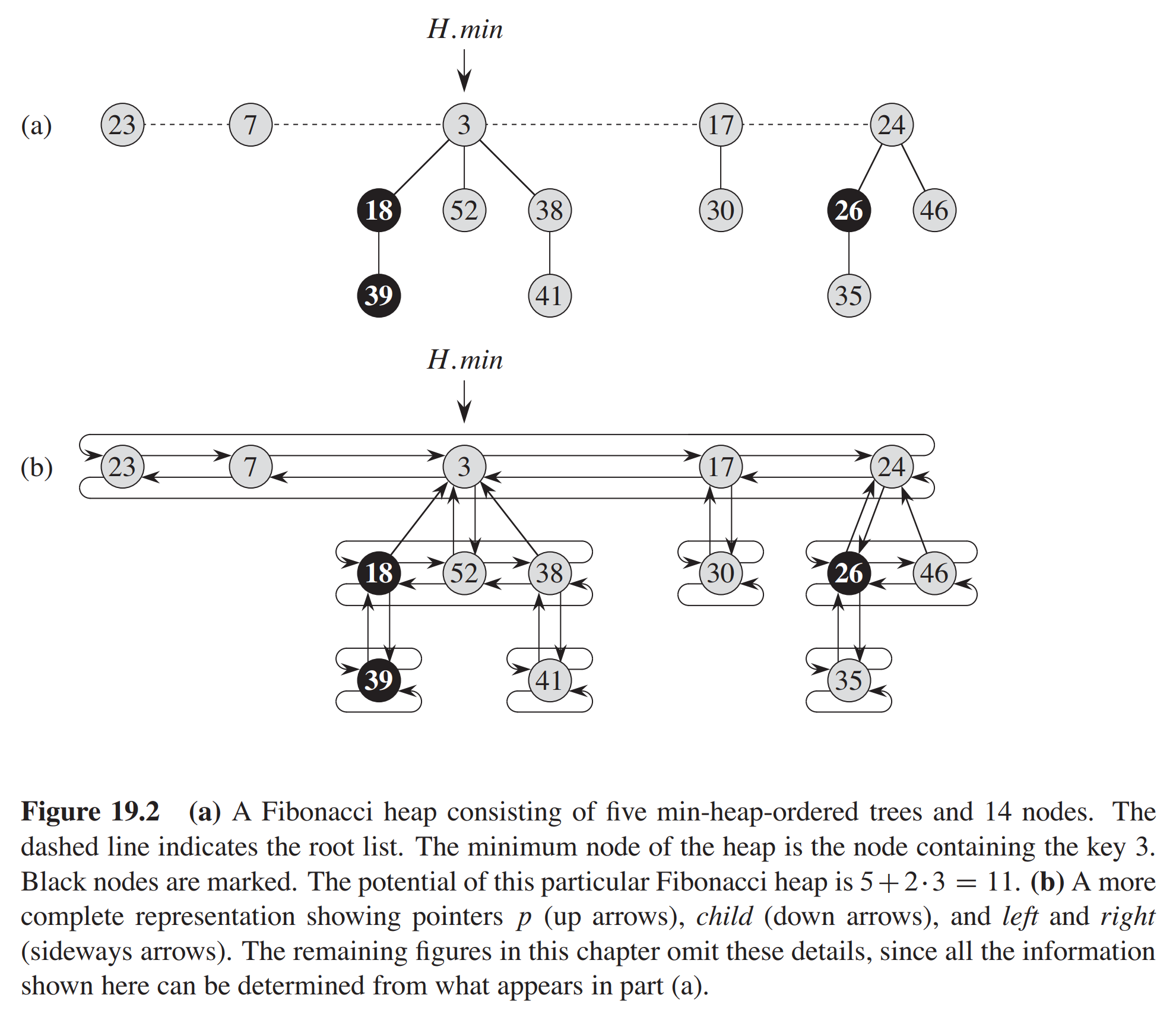
As the figure shows, each node $x$ contains a pointer $x.p$ to its parent and a pointer $x.child$ to any one of its children. The children of $x$ are linked together in a circular doubly linked list, which we call the $child list$ of $x$. Each child $y$ in a child list has pointers $y.left$ and y.right that point to $y$’s left and right siblings, respectively. If node $y$ is an only child, then $y.left=y$, $y.right=y$. Siblings may appear in a child list in any order.

With the help of circular, doubly linked lists, we are able to:

1. Insert a node into any location or remove a node from anywhere in $O(1)$ time.
2. Concatenate any two given lists into one circular, doubly linked list in $O(1)$ time.